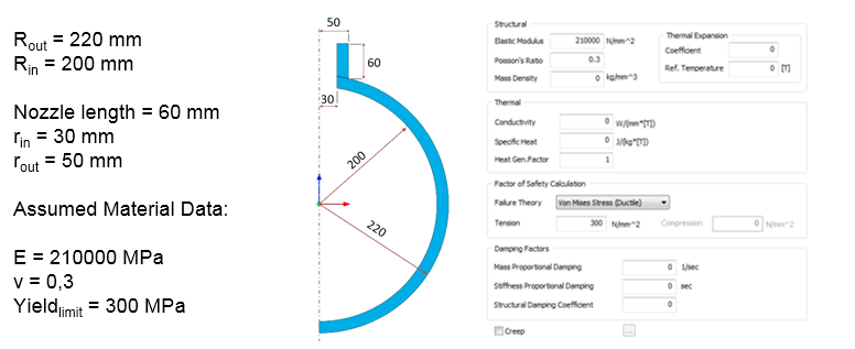
- Introduction
Thin wall pressure vessels are widely used in industry for storage and transportation of liquids and gases. Most of such pressure vessels are either cylindrical or spherical:

A sphere is the optimal geometry for a closed pressure vessel because it is the most structurally efficient shape of both.
This document provides an example of numerical analysis for a small spherical pressure vessel with an external cylindrical nozzle.
This problem can be analyzed in 3 different ways and the purpose of this document will be to compare the results obtained from those 3 shapes:
- Axisymmetric Solid model
- Model with 2D shell elements
- Model with 3D solid elements
- Modeling in midas NFX
2.1. Geometry
Geometry model can be created directly or imported to midas NFX from an external CAD software. Less complex geometries can be created directly using the tools for geometry generation.
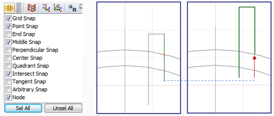
Sketch translation with snap to intersecting curves.
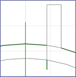
Intersected curves for 2D face creation
2.1. FE Model
Midas NFX uses the imported geometry as the base of the FE Model. Midas NFX allows working directly on curves, 2D surfaces or solids. FE model can be associated or not with the geometry, depending on the choice of the FEA Analyst. Working with mesh elements directly allows more flexibility for advanced users. Mesh elements can be extruded, revolved and properties can be modified. The geometry of a spherical pressure vessel allows modeling with asymmetrical elements, 2D shells and solids.
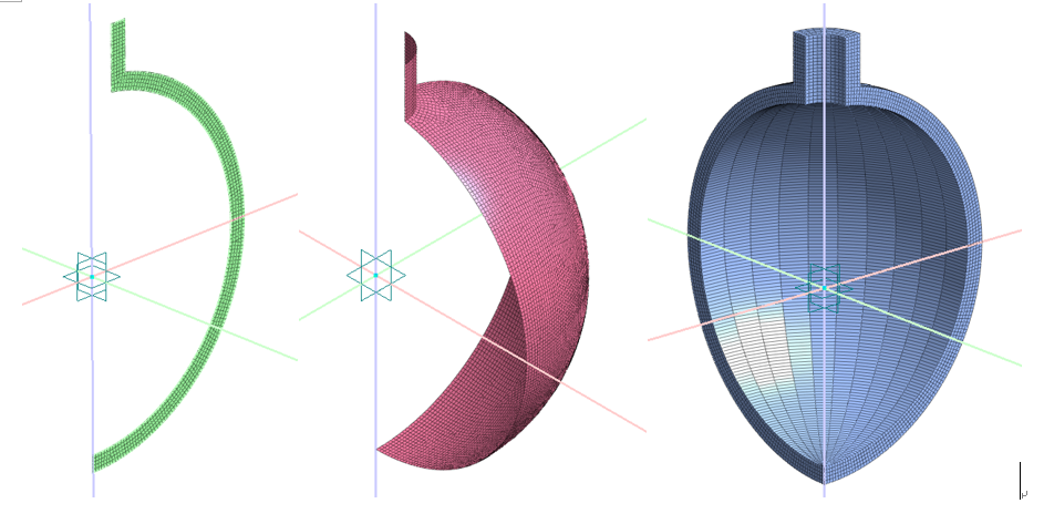
Axisymmetric model created on 2D face (Left), 2D Shell model created on mid-surface from 3D geometry (middle) and 3D Solid mesh model (Right) created by mesh revolve command
2D Shell Spherical pressure vessel:
2D Axisymmetric Spherical pressure vessel: 3D Solid Model:
2.2. Loads and Boundary Conditions
Each type of FE representation requires proper constraints and load assignment. Midas NFX offer a wide variety of loads which can be applied to geometrical entities such as points, curves, surfaces or directly on nodes or elements. One of the most important steps in finite element analysis is to apply the proper constraints. For 2D and 3D axisymmetric models with pressure loading, we use symmetric definition. In case of presented 2D axisymmetric model, point constraint will require balancing from loading.

Working on mesh requires different tools for loading and boundary condition application. Pressure application can be slightly more difficult to be assigned, especially for complex shapes and high number of elements. Selection features are very helpful for quick and effective element selection for loading condition application, especially the “Select Neighboring Edges” feature.
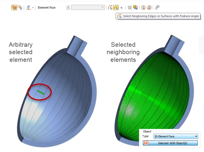
Selection of 3D Faces for Pressure loading
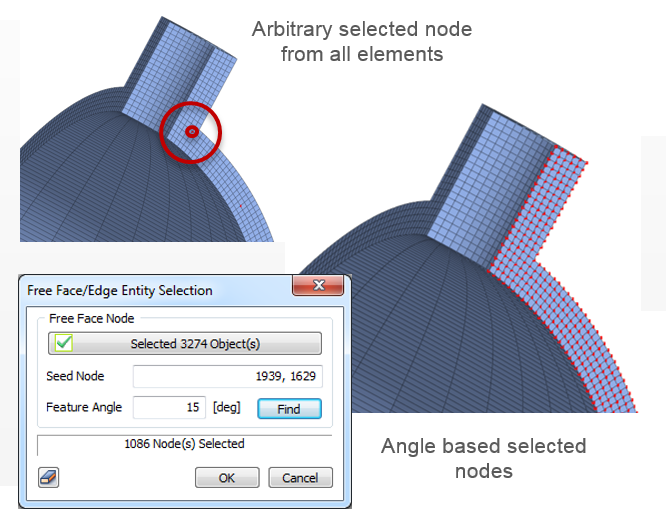
Node selection for side constraining
Results Verification and Displaying
1. Results Comparison
Different FE Models lead to results with different level of accuracy and require different post-processing techniques to extract efficiently the results. Results obtained look similar, but an attentive investigation and comparison of the results is generally required before taking any important decision.
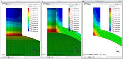
Von Mises output contour for all FE models
- 2. Reactions Summation
The investigation of the reaction forces on the constrained areas and nodes shows that the reaction Force RZ is almost the same as the applied force F
Reaction RZ = 703.95 * 4 = 2815,8 N
Force F = 1/2827.43 = 2827,43 N
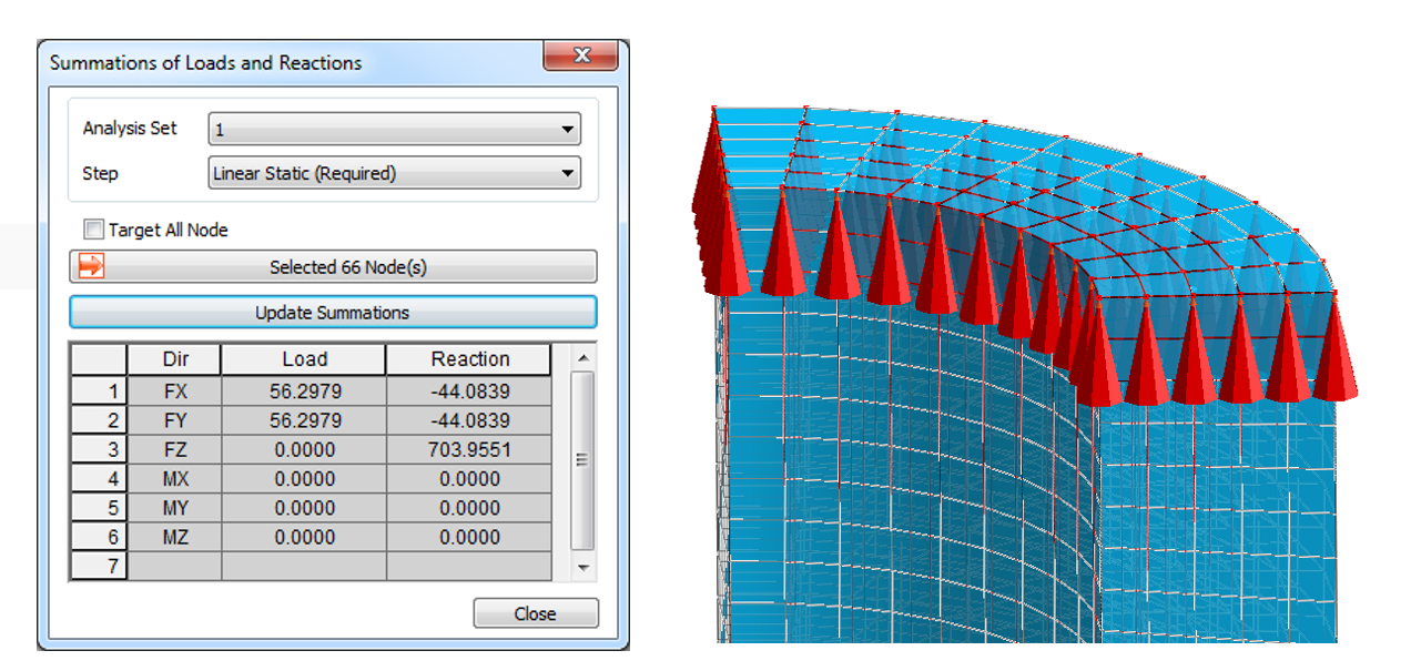
Reaction Summation
- 3. Stress Linearization
Stress categorization is very important in pressure vessel calculation. This is where stress linearization is used to extract the nodal data of complex stress patterns that appear along the thickness line. It allows to break down total stress into the following components:
– Membrane Stress
– Bending Stress
– Membrane + Bending Stress
– Peak Stress
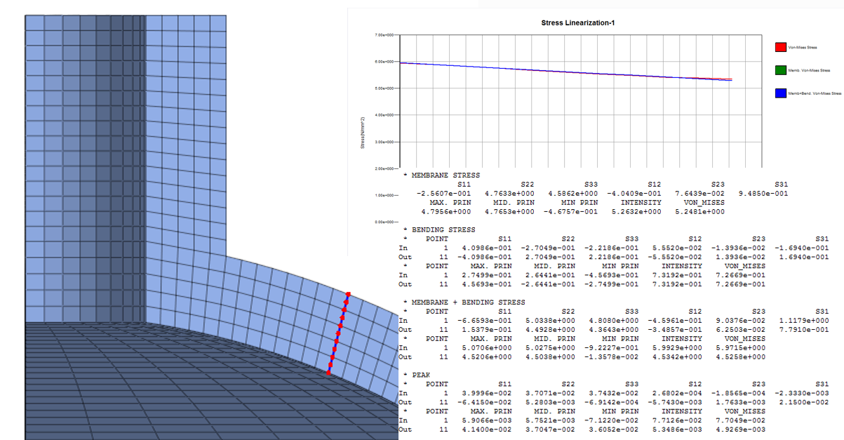
Stress Linearization across the thickness of vessel
GET THE FREE GUIDE
24 Links and Articles to know about Pressure Vessel Design and Simulation